The Challenge

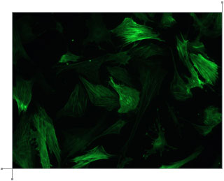
Dr. Masaaki Yoshigi is an MD, a Ph.D., a former Huntsman Cancer Institute researcher, and a LabVIEW programmer. David Moore met Dr. Yoshigi at NIWeek 2000 where he presented a paper on his work growing mouse heart cells on a flexible sheet as the sheet is stretched. If you stain and photograph the cells correctly, the actin fibers that form the skeleton of each cell become visible. The fibers tend to align with the direction of stretching, and Dr. Yoshigi was trying to analyze that alignment from the images he captured. He had a technique (based on Fourier transforms) that would give one result for a whole image, but he really wanted to know about individual cells, so he asked anyone with suggestions to contact him.

David Moore immediately had a “Good Idea.” The solution was to use brightness gradients, shown as vectors in the image to the left, to measure individual fiber directions. That would give Dr. Yoshigi even more detail than he was hoping for.  

But how do you measure gradients efficiently in an image? The LabVIEW IMAQ library contains all the functions you need. The Convolute function, used with a Sobel filter kernel, can be used to measure either the horizontal or vertical component of the gradient. Combine the horizontal and vertical components and you have the full gradient vector. In IMAQ, you can store horizontal and vertical as the real and imaginary components of a complex number image. Below is the example code in LabVIEW.

Innovative Presentation

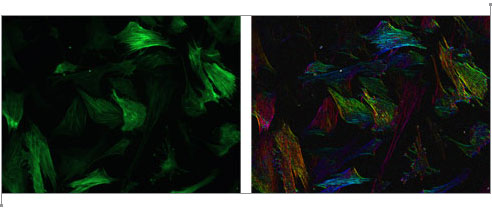
Although an “image” consisting of complex numbers is handy for storing the gradient data, it’s not something you can actually look at. David next created a color image, where the brightness was determined by the magnitude of the gradient vector and the hue was determined by the direction. As you go around the circle of directions, every hue shows up twice, so that the two sides of a fiber will both be the same color as represented by gradient vectors and their corresponding colors to the right. Below is a sample of the raw image, and the result after the “directional stain” has been applied. As you can see, each fiber is colored according to its direction. Click the image to view a close-up of stained fibers.

Moore Good Ideas

Dr. Yoshigi loved the result of directional staining, but David recognized that there was still one more innovative analysis needed before the pretty qualitative picture could be turned into real quantitative data. What would happen when Dr. Yoshigi tried to find the average direction of the fibers for a cell? The gradient vectors that were in opposite directions would cancel each other out, and the result would always be zero!

Before you take the average, you need to map your data from gradient vectors that color like the image to the left to something else that maps like the image to the right where the two sides of each fiber give the same vector. Once you know that that’s the result you want, it’s really easy to do mathematically: you just square the numbers before you average them.

With innovative analysis and presentation from Moore Good Ideas, Inc., Dr. Yoshigi went from the approximate results he had to the real quantitative data he wanted and beautiful qualitative images he never expected.